Database Index: Part 3 - Under the Hood - PostgreSQL's B-Tree in Action

A step-by-step dive into PostgreSQL’s B-Tree internals — from index pages to heap tuples — with real queries, byte-level insights, and visual guides.

Aug 14, 2025

The Reality Check🧵

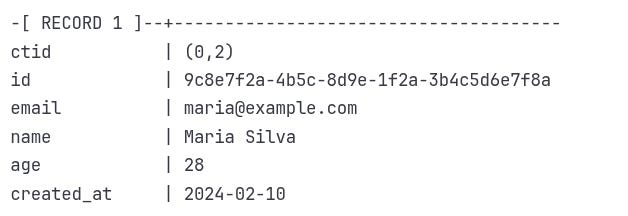
In Part 2, we traced Maria's email through a conceptual B-tree in milliseconds. We observed the database navigate from the root page to the leaf page, follow a row locator, and deliver her complete record with surgical precision.

But you might be thinking: "That's a nice theory, but how does PostgreSQL actually do this? What does real production code look like?"

Time to find out.

We'll run the same query on a real PostgreSQL database, use developer tools to inspect its internals, and compare the practical implementation to our conceptual model. Spoiler: PostgreSQL's B-tree implementation closely matches our description from Part 2, with additional optimizations, handling of edge cases, and real-world complexities.

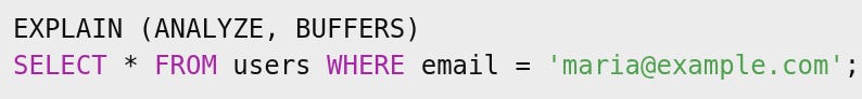
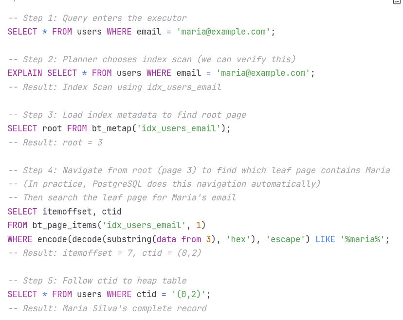
Let's start with that same query — but this time, let's see what PostgreSQL actually does:

Output:

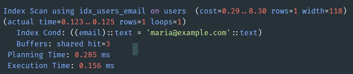
0.156 milliseconds. Maria's record was retrieved from a table with potentially millions of rows.

But what occurs during those three buffer hits? What is meant by a "shared hit'? And how can we inspect those pages to observe the actual B-tree navigation discussed in Part 2?

Today, we're going behind the abstraction layer.

Setting Up Our Investigation Lab 🧪

Before we start dissecting PostgreSQL's internals, you'll want to follow along. I've prepared a complete Docker environment that recreates the exact scenario from Part 2, with all the necessary PostgreSQL extensions and debugging tools pre-installed.

# Clone the demo environment
git clone https://github.com/cmsandiga/makotons_substack.git
cd postgresql-btree-internals

# Start PostgreSQL with debugging tools
docker-compose up -d

# Connect and verify Maria exists
docker exec -it postgres_pageinspect_demo psql -U makotons -d makotons_substack -c "SELECT * FROM users WHERE email = 'maria@example.com';"```

What this gives you:

PostgreSQL 16 with pageinspect extension
Pre-loaded with the exact users table from Part 2
pg_filedump for binary file analysis
Sample data structured to create the B-tree we discussed

Don't worry if you can't run this right now - I'll show you all the outputs and explain what each command reveals. But if you want to experiment as we go, the environment is ready.

1: The File System Reality

How PostgreSQL Organizes Itself

Before we can find Maria's data on disk, we need to understand how PostgreSQL keeps track of everything. Where does it store information about databases, tables, and indexes?

PostgreSQL's Metadata System

PostgreSQL stores information about your databases, tables, and indexes in special system tables called catalogs. These are regular tables that PostgreSQL uses to manage itself - metadata about your metadata.

System Catalogs:

pg_database: Information about every database in the PostgreSQL cluster
pg_class: Information about tables, indexes, views, and sequences within the current database
pg_attribute: Column definitions for each table
pg_index: Index definitions and their relationships to tables

PageInspect Extension:

But system catalogs only tell us about the logical structure. To see what's actually inside the B-tree pages, we need a special extension called pageinspect.

Think of pageinspect as PostgreSQL's "X-ray machine" - it lets you see inside the binary page structure that's normally hidden from users. Without it, pages are just opaque 8KB blocks of data.

PageInspect functions we'll use:

bt_metap(): Shows B-tree metadata (root page, tree height, etc.)
bt_page_stats(): Shows statistics for individual B-tree pages
bt_page_items(): Shows the actual items stored in B-tree pages

External debugging tool:

pg_filedump: Command-line tool for examining raw binary file content (works outside PostgreSQL)

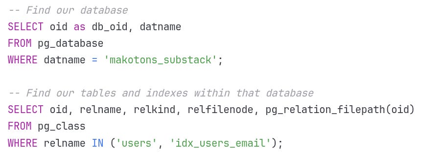
Today, we'll focus on pg_database and pg_class to map our conceptual files to actual disk storage, then use the pageinspect functions to examine the B-tree structure.

The catalog hierarchy:

Output:

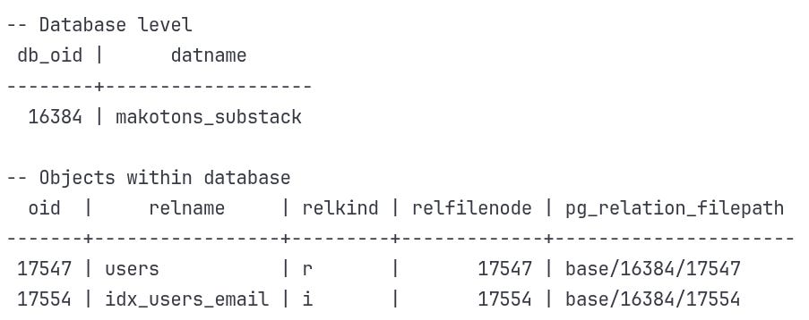
Key information 🔑:

relkind: 'r' = table (relation), 'i' = index
oid: PostgreSQL's internal logical identifier
relfilenode: The actual file number on disk

Why two identifiers?

Most of the time oid and relfilenode are the same, but they serve different purposes:

oid: Never changes, used for internal references
relfilenode: Can change during operations like VACUUM FULL or REINDEX

This separation lets PostgreSQL rebuild files without breaking internal references.

Where PostgreSQL Actually Stores Your Data 📂

Now we can map these numbers to actual files on disk:

The file system hierarchy:

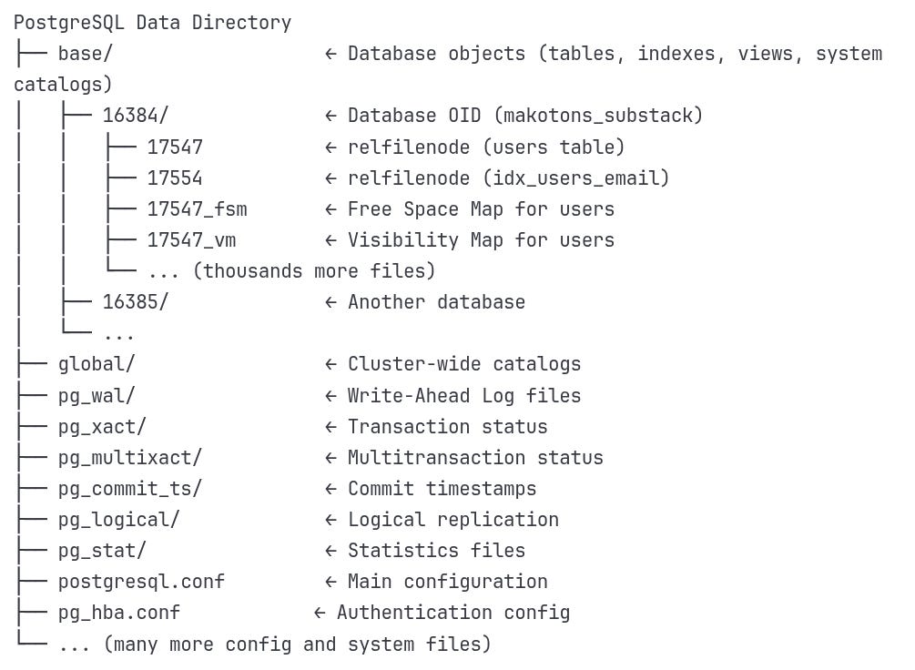
So our files are actually:

Users table: /var/lib/postgresql/data/base/16384/17547
Email index: /var/lib/postgresql/data/base/16384/17554

Examining the Physical Files

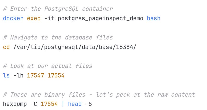
Output:

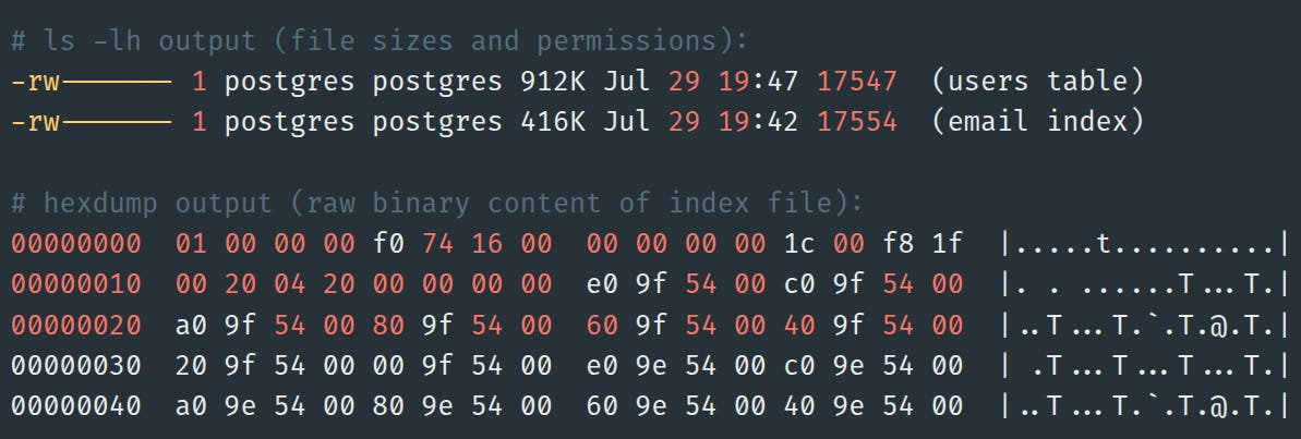
Size Analysis:

Table file: 912 KB for complete user records (UUID + email + name + age + timestamp)
Index file: 416 KB for just emails + pointers (55% smaller!)

This size difference is exactly what we predicted in Part 2. The index doesn't duplicate data - it creates a lightweight navigation structure.

🍖 This is the actual binary B-tree data! Each byte has meaning - page headers, item pointers, tuple data. But raw hex is hard to parse. That's where PostgreSQL's debugging tools come in.

2: Opening the Black Box with pageinspect

Index Metadata: Locating the Root Page

Before we can navigate a B-Tree, we need to locate its root. PostgreSQL stores that information in the metapage, always at page 0 of the index file. Think of it as the header of the file, like a file system superblock.

PostgresSQL

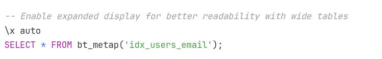
Output

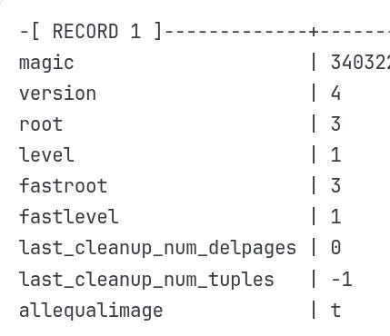
Key Information:

magic = 340322: PostgreSQL's B-tree signature (like a file format identifier)
root = 3: The root page is page #3 in the index file
level = 1: This is a 2-level tree (root + leaf pages)
version = 4: B-tree format version

🍖 In PostgreSQL B-Trees, the root is simply the topmost page, and it isn’t fixed to page 1.
Page 0 is always the metadata page (BTMetaPage), which stores the root’s block number.
The first data page (block 1) starts as both root and leaf.
When that page splits, PostgreSQL allocates the new right leaf (block 2) first, and then an internal root (block 3) that points to both leaves.
In bulk builds, all leaf pages are written first, and the root is allocated after them — often ending up at the last block + 1.

Loading the root page to see the navigation structure

Now that we know the root might not be page 1 — and in our case it’s block 3 — let’s inspect that page directly to understand its role in the tree.
Using bt_page_stats, we can see whether it’s a leaf or an internal page, and how it points to its children.

PostgresSQL

Output:

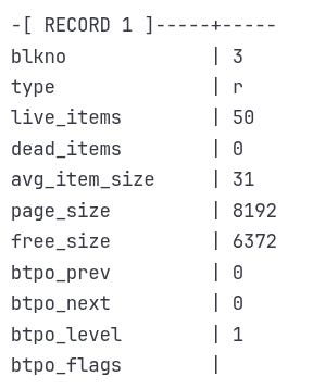
Key Information:

type = 'r': This is the root page.
('r' stands for root; PostgreSQL uses this label in bt_page_stats to differentiate it from normal internal pages 'i'.)
btpo_level = 1: Confirms this is an internal node, not a leaf.
live_items = 50: It contains 50 pointers to child pages (probably leaf pages).
free_size = 6372: Only ~1.8 KB is used — room for more pointers.

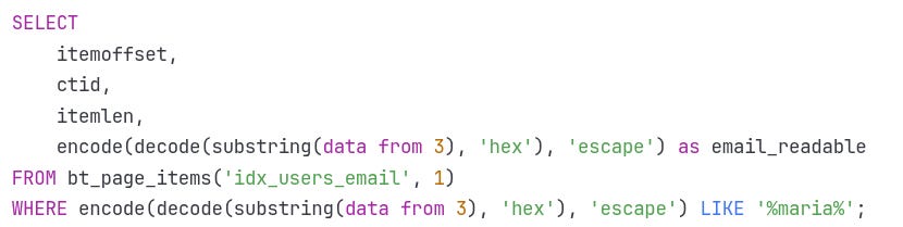
Scanning the leaf page for 'maria@example.com'"

In the previous step, we saw that the root is an internal page pointing to several leaves. Now, we’ll follow one of those pointers to a leaf page (block 1 in our example) and inspect its contents.
Leaf pages contain the actual index entries — the key values along with their tuple identifiers, known in PostgreSQL as ctid (current tuple IDs).
By scanning this page and filtering for maria@example.com, we can confirm exactly how the index stores and locates this key.

PostgresSQL

Output

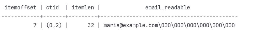
Perfect! We found Maria exactly where our conceptual model predicted:

itemoffset 7: She's the 7th item on this page (matches our Part 2 example)
ctid (0,2): Row Locator pointing to page 0, slot 2 in the users table.
32 bytes: Each index entry is exactly 32 bytes
Email data: The actual email with null padding for fixed-width storage

This mirrors our Part 2 path—next, we’ll decode the row locator (ctid) that points into the heap page and slot.

What’s a heap table?

In PostgreSQL, a heap table is the actual on-disk storage for table rows.

It’s made of fixed-size pages (usually 8 KB) that contain the physical row data.
Rows are stored in no particular order — the heap is unordered.
An index doesn’t store the entire row; it stores the search key plus a ctid pointing to the row’s exact location in the heap.

The ctid contains:

Block number → which heap page the row is on
Offset number → which slot in that page holds the row

🍖 Why is it called a “heap”? Here, “heap” follows classic database terminology for an unordered file of records. It does not mean a heap data structure (priority queue) or heap memory in programming. The name comes from early DBMS literature, where “heap file” meant “records stored wherever there’s space, without sorting by key.”

Understanding the ctid (Row Locator)

In PostgreSQL, the ctid (current tuple ID) is the bridge between the index and the actual table row. Every index entry contains a ctid, which is the physical location of the tuple in the heap: the block number (which page of the table) and the offset (which slot in that page). When we query the table by index, PostgreSQL uses this pointer to jump directly to the correct heap tuple, then checks visibility before returning it.

The ctid is PostgreSQL's implementation of our "Row Locator" concept from Part 2. It's a 6-byte structure:

4 bytes: Block number (page identifier)
2 bytes: Offset number (tuple position within page)

PostgresSQL

Output:

🍖 Every PostgreSQL table automatically has a hidden system column called ctid.
You won’t see it in \d output, but it’s always there. PostgreSQL uses it to identify the physical location of each row as (block_number, offset).

We’ve reviewed the lookup in slow motion. Next, let’s combine it into a single visual — our conceptual path from Part 2 aligned with PostgreSQL’s actual commands and outputs.

3: The Complete Journey Visualization

Let's trace the complete path from our query to Maria's data, showing both the conceptual model from Part 2 and the PostgreSQL reality:

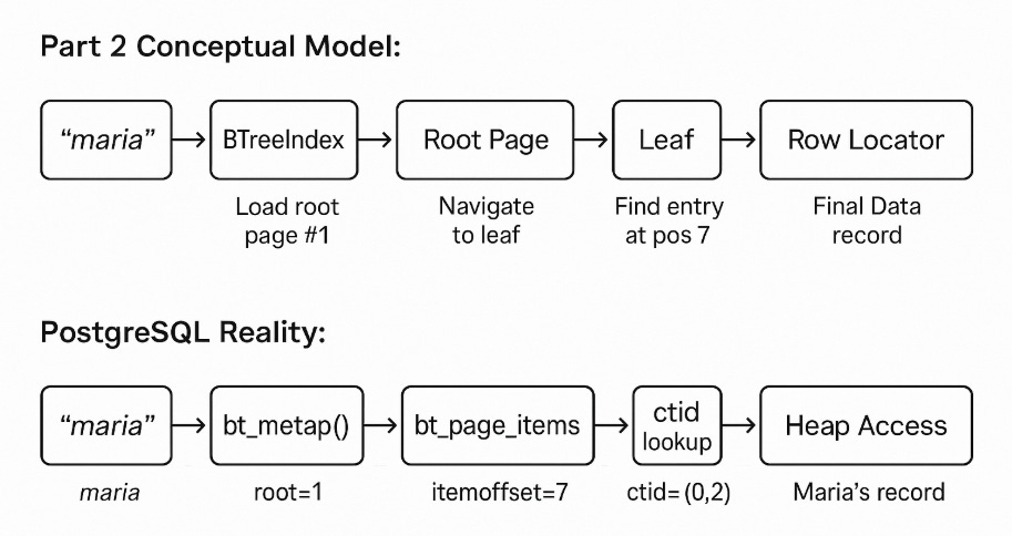
This journey confirms what we modeled in Part 2: PostgreSQL's index navigation isn't just theoretical — it’s real, reproducible, and can be inspected down to the byte level.

By combining bt_metap(), bt_page_items(), and ctid lookups, we traced a full query through root, leaf, and ultimately to the exact row in the heap, just as we predicted — only now, with actual disk pages and offsets. However, one important detail remains: in our model, we assumed every page is read from disk. In practice, PostgreSQL is much smarter — it uses memory to avoid unnecessary I/O. Let's explore how that works.

If you’ve enjoyed the journey so far, share this article with friends or colleagues who love digging into database internals.

4: Buffer Management - The Production Reality

One key difference between our Part 2 model and PostgreSQL is how pages are stored in memory. We simplified it as "load page from disk," but PostgreSQL uses a complex buffer pool system.

Understanding Buffer Hits

Remember this from our EXPLAIN output?

Buffers: shared hit=3

This means PostgreSQL accessed 3 pages, but all were already in the buffer pool (shared memory). No disk I/O was needed!

Buffer Pool Visualization:

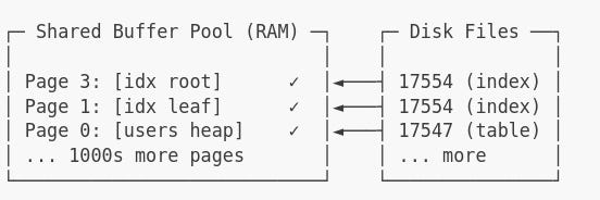
PostgreSQL's buffer pool is backed by shared memory — typically configured using the shared_buffers parameter.

This defines how many 8KB pages PostgreSQL can cache in RAM. Default: ~128MB

🍖 What happens when the buffer pool fills up?
PostgreSQL uses a clock-sweep algorithm — a smart variant of LRU (Least Recently Used) — to evict less-accessed pages and make room for new ones.
Hot pages that are frequently read tend to survive. Cold, stale pages eventually get swept out.

Cold start Output

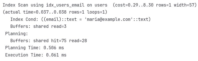
Those 75 buffer reads during planning come from system catalogs like `pg_class`, `pg_statistic`, and `pg_attribute`. PostgreSQL accesses these to decide if using an index is worthwhile, all before executing the query.

Warm Cache Output:

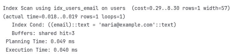
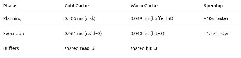
In the end, 3 index pages were accessed in both cases — but in the warm run they came from RAM (0.040 ms execution), while in the cold run they came from disk (0.061 ms execution). The larger 0.506 ms difference you see is from planning, which also benefits from hitting cached catalog pages instead of reading them from disk.

🍖 Internally, PostgreSQL reports buffer usage like:
shared read=N → block read from disk
shared hit=N → block found in buffer cache
So “3 blocks from disk” = “shared read=3”

That’s the meat 🍖 of buffer hits — they measure whether PostgreSQL is fetching from memory or disk.

☝️Curious about the rest of the EXPLAIN (ANALYZE, BUFFERS) output?
Drop a comment and I’ll prepare a dedicated post walking through every field in detail.

5: Binary Data Deep Dive

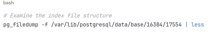
Let's examine what those pages contain at the byte level. PostgreSQL provides pg_filedump for forensic analysis of the raw binary data.

Index File Analysis

Sample Output:

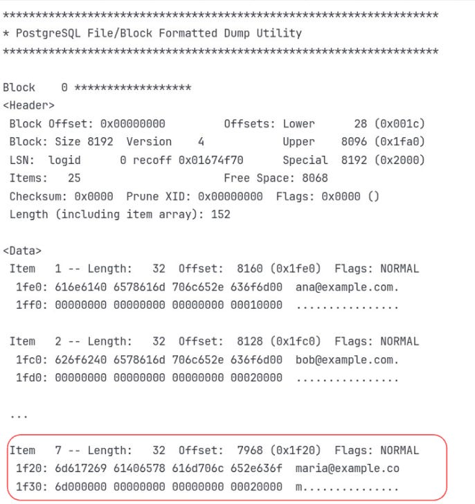
Key Insights:

Item 7: Maria's entry at byte offset 7968
Binary layout: maria@example.com in ASCII, followed by the ctid (0,2)
Fixed size: Each entry is exactly 32 bytes
Null padding: Extra bytes filled with zeros for alignment

Page Header Anatomy: How PostgreSQL Organizes an 8KB Page

Every PostgreSQL page — whether it's from a table or an index — starts with a 24-byte header. This isn't visible in your `bt_page_items()` output, but it's always there, quietly organizing everything.

Here's what it includes:

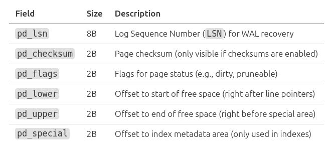
In pg_filedump, these fields are shown as Lower, Upper, Special, and LSN — exactly what you’d find at the start of an 8KB page.

These values allow PostgreSQL to:

- Track where new tuples can fit (`pd_lower` and `pd_upper`)

- Know when a page is full or fragmented

- Reserve space for metadata (especially in index pages)

Think of it as the **table of contents** for the page: PostgreSQL doesn’t scan blindly — it uses these offsets to locate where every tuple or index item lives surgically.

Decoding the ctid

The last 6 bytes of Maria's entry contain the ctid:

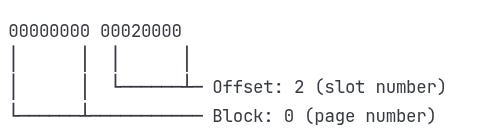
This binary data encodes ctid (0,2), which points to page 0, slot 2 in the users table.

Heap File Analysis

We’ve decoded the ctid from the index — now it’s time to follow it straight into the heap table.
Using pg_filedump, we’ll inspect the exact heap page (page 0) and slot (2) where Maria’s record lives, confirming that the row locator we found in the index really does point to her complete row on disk.

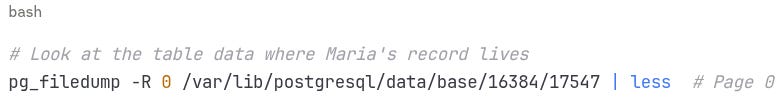
Output (simplified):

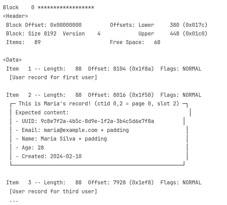
Perfect match! The ctid (0,2) from the index correctly points to slot 2 on page 0, where Maria's complete 88-byte record lives.

From Mystery to Mastery

When we started this journey, finding Maria's record in milliseconds felt like magic.
But it’s not magic — it’s engineering, layered over decades of computer science.

You've now seen how PostgreSQL turns theory into action:

File Structure – Real binary files with predictable layouts
Page Management – Sophisticated buffer pools and memory optimization
Navigation – B-tree traversal with concurrency built in
Row Locators – Direct addressing through TIDs and ctid

More importantly, you now have the tools to peek under the hood of any database engine.
Tools like EXPLAIN, pageinspect Raw binary inspection isn’t just for academics — it’s how you debug, optimize, and gain a deeper understanding.

If you’ve made it this far, you’re not just using databases — you’re thinking like one.
And today, we’ve truly come full circle: from the big-picture theory in Part 2 to inspecting real bytes on disk, following PostgreSQL’s exact path through pages, pointers, and rows.

👉 If we hit 3 comments, the next deep dive will cover index bloat and how PostgreSQL handles it.

Makotons Substack

Discussion about this post

Ready for more?