
Database Indexes: Part 2 — How B-Tree Indexes Work Internally (With a Real Query Walkthrough)
Ever wonder how databases locate one record among millions in just milliseconds? This deep dive traces a real query through every layer of B-tree architecture—from root pages to raw bytes.

A Millisecond Mystery
You're running a query on a table with 10 million users. You type:

And almost instantly, the row appears. Not seconds, not even a full blink — just milliseconds.
How is that even possible?
If we had to read the table record by record, it would take minutes. But under the hood, the database engine performs a dance of jumps, skips, and direct page reads. The secret behind this speed?
A humble yet powerful structure: the B-tree index.
Quick Bridge from Part 1
In Part 1, we saw how databases evolved from sequential files to B-trees to solve the linear search problem. Now it's time to see exactly how a B-tree delivers those millisecond responses.
Time to open the black box and see what happens inside.
Missed Part 1? Don’t worry — this deep dive stands on its own, but feel free to circle back later to understand how we got here.

Following Maria's Email Through the B-Tree
Let's trace this exact query through every step:
The Complete Path:
Query → BTreeIndex → Root Page → Leaf Page → Row Locator → Final DataWe'll see exactly what happens in memory, on disk, and how they transform into each other.
🔑 Key Concepts First
Before we dive into the journey, let's quickly understand the main concepts we'll encounter:
What is a B-Tree?
A B-tree is similar to a multi-way decision tree, where each node can have multiple children (not just two, as in binary trees). Think of it as a book with a detailed index where:
Each index entry (node) contains multiple topic ranges (keys)
Each topic range guides you to the right section or specific page
You can skip entire sections with each decision
Key Properties:
Always balanced - All leaf nodes are at the same depth
Wide, not tall - Nodes contain many keys (50-200+ per node)
Ordered - Keys within each node are sorted
Self-maintaining - Automatically stays balanced during inserts/deletes
Visual Structure:
            [100]                   ← Root node
           /     \
     [50 | 75]   [150 | 200]        ← Internal nodes
     /   |   \    /   |    \
  [10] [60] [80] [120] [160] [250]  ← Leaf nodes with actual data
Each internal node acts like a "signpost" that says:
Root: everything < 100 goes left, ≥ 100 goes right
Left internal: < 50, 50-74, ≥ 75
Right internal: 100-149, 150-199, ≥ 200
Why This Structure Matters:
Height stays low: A 3-level B-tree can handle millions of records. Compare this to a binary tree that might need 20+ levels for the same data.
Disk-friendly: Each node fits exactly in one 4KB page, so every "decision" requires just one disk read.
What is a BTreeIndex?
Think of it as a separate file (users_email.idx) that acts like a "smartphone book" for your tablet. Instead of names→phone numbers, it maps emails→exact locations where those user records live.
What are "Pages"?
Both index and data are stored in 4KB chunks called "pages" - like pages in a book. Each page has a unique number (Page #1, Page #47, etc.) so the database can jump directly to any page without reading everything before it.
Why 4KB pages?
This matches how your hard disk and operating system prefer to read data - one efficient chunk at a time, not byte by byte. It's like reading a paragraph instead of one letter at a time.
Memory ↔ Disk Transformation
You'll see "Memory" and "Disk" side-by-side throughout our journey:
In Memory: Objects with properties (
BTreeNode.keys,BTreeNode.children)On Disk: Raw bytes stored in files (
0x6d 0x61 0x72...)
The database constantly transforms between these: read from disk → deserialize into objects → work in memory → serialize back → write to disk.
Now let's see how these concepts work together in practice...
🔍Step 0: Understanding Our Data
Before we search for Maria’s email, the engine first needs to understand what kind of table it’s dealing with — its shape, structure, and what fields exist.
What is our Users Table?
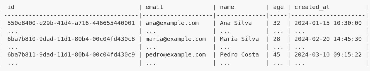
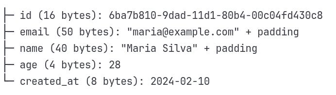
First, let's see what we're indexing. Our users table looks like this:
id: UUID identifier
email: user's email address
name: user's full name
age: user's age
created_at: timestamp
An Index: Build B-tree on email field for fast lookups
Sample data:
What happens on disk:
When you create this table and index, the database creates two separate files:
users_data.bin- The actual table dataContains all user records (id, email, name, age, created_at)
Organized in 4KB pages for efficient reading
This is where your actual data lives
users_email.idx- The email indexContains only email addresses + pointers to the data file
Much smaller than the data file
Organized as a B-tree for fast searching
File System:
├── users_data.bin    (10MB - user records)
└── users_email.idx   (2MB - just emails + pointers)
📌 Note: This article focuses on the **logical layout** of B-tree indexes — how they map keys to data pages. We’re not diving into insertion, deletion, or rebalancing algorithms here — not because they’re boring (they’re not!), but because many excellent articles already cover them well.
Enjoying the deep dive? Feel free to share it
Step 1: Loading the Root Page
What the Database Does:
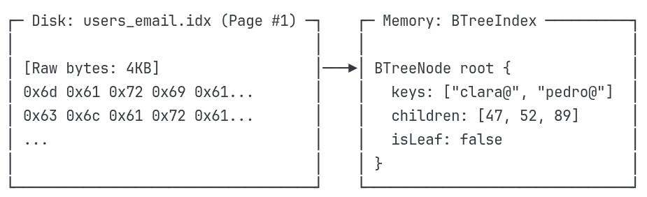
Open the index file: users_email.idx
Read page #1 (4KB) from disk
Deserialize bytes into BTreeNode object
Step 2: Navigation Logic
Understanding the Structure We Just Discovered
Now that we've loaded the root page, we can see the navigation paths available to us:
What this structure tells us:
The path we'll take - Root → Page #52 → Maria's record
Page numbers aren't sequential - #47, #52, #67 could be scattered across the disk
We only load what we need - We've loaded Page #1 (root), and will only read Page #52 from disk into memory next, leaving #47 and #67 as untouched bytes on disk
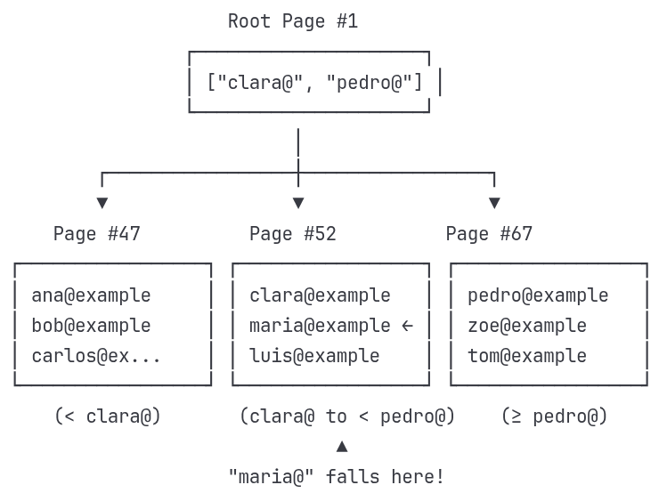
Navigation boundaries - The root keys ["clara@", "pedro@"] divide the data space into ranges
B-Tree Decision at the Root
To decide which child page to follow, the B-tree compares our target email with the boundary keys in the root node:
Target: "maria@example.com"
Root keys: ["clara@", "pedro@"]
We go step by step:
Compare with "clara@"
"maria@" >= "clara@"→ ✅ Yes → So it's not in the leftmost child (Page #47)Compare with "pedro@"
"maria@" < "pedro@"→ ✅ Yes → So it's before the "pedro@" boundary
Together, these comparisons tell us:
"maria@" falls in the middle range: ["clara@", "pedro@")
This means we navigate to:
→ children[1] = Page #52Note: B-trees use half-open intervals — ranges that are inclusive on the left and exclusive on the right. So the middle child is responsible for any key ≥ "clara@" and < "pedro@".
Step 3: Loading the Leaf Page
Understanding Internal vs Leaf Pages
We're about to encounter two different types of pages in our B-tree:
Internal Pages (like the root): Act like a "table of contents"
Store boundary keys that divide data into sections
Point to other pages (either more internal pages or leaf pages)
Don't contain actual email addresses - just navigation guides
Leaf Pages: Store the actual index entries
Contain the real email addresses we're searching for
Point to actual data locations (not other pages)
This is where we'll finally find "maria@example.com"
Think of it like a library:
Internal pages = Floor directory ("Science books: Floor 3")
Leaf pages = Shelf labels ("Biology: Books A-M on this shelf")
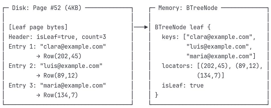
Disk Read Result:
Step 4: Finding the Exact Match
We already loaded Page #52 and saw its memory structure:
keys:     ["clara@example.com", "luis@example.com", "maria@example.com"]
locators: [(202,45), (89,12), (134,7)]
Now it’s time to match our search target.
Searching in the Leaf Page
The database now performs a linear scan inside the node — but only within that tiny 4KB page.
It compares each stored key with your target:
Target key: "maria@example.com"
1. "clara@example.com" → ❌ not a match
2. "maria@example.com" → ✅ match found!
Once matched, it returns the Row Locator:
RowLocator result:
├─ page_id: 134     ← Points to the data file page
├─ slot_id: 7       ← Record’s slot within that page
The index never stores the actual user row. It just tells you exactly where to find it.
The Row Locator acts like GPS: it leads the engine directly to Maria’s record in the data file — without touching anything else.
Step 5: Final Data Access
Understanding Index vs Data Storage
We're about to jump from the index file to the actual data file. These are stored separately:
Index File (users_email.idx): Contains only navigation info (keys + pointers)
Like a library catalog that tells you where books are located
Small and fast to search through
Doesn't contain actual user data
Data File (users_data.bin): Contains the actual user records
Like the actual books on library shelves
Large file with all the real data
Organized in 4KB pages for efficient access
The Row Locator (134,7) is like a call number that takes you from the catalog to the exact shelf and book you want.
Row Locator Usage:
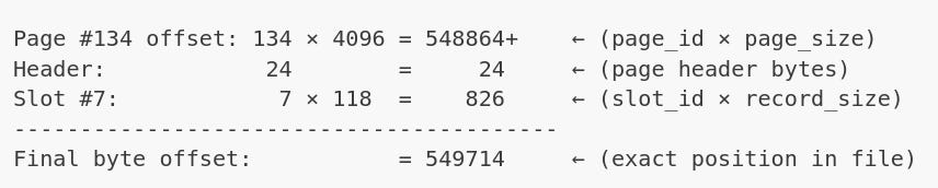
Using (page=134, slot=7):
Open data file:
users_data.binseek(data_file, page_134_offset)Calculate slot offset:
24 + (7 × 118) = 850 bytesread(118_bytes)from that position
Data Page Structure:
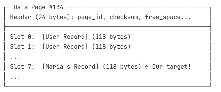
Record Layout (118 bytes each):
Reality Check: Binary Storage on Disk
So far we've shown conceptual examples — nodes, keys, and locators. But when the database hits the disk, there are no JSON objects or structs waiting to be read.
Everything is just bytes — raw, fixed-size, and precisely arranged.
When the database receives a row locator like (134, 7), it doesn't need to search or parse. It does one thing: math.
What is seek()?
seek(offset) is a system call that tells the operating system:
“Move the read pointer in this file to byte position X. Don’t read anything yet — just get ready.”
Why seek() works so efficiently
Because every part of the layout is predictable:
Pages are fixed at 4KB → easy to compute start offsets
Records are fixed at 118 bytes → slot math is trivial
No variable-length gaps → no need to read forward to find boundaries
No scanning, no parsing, no disk traversal. Just a mathematical jump.
Why it’s so fast
Files are byte-addressable
All files are just sequences of bytes. Your OS sees a file like this:
[0][1][2]...[827400][827401][827402]...So when you say seek(827400), the OS moves the internal read pointer there instantly.
No I/O happens during
seek()seek()itself doesn’t read — it only positions the pointer.
Actual disk I/O happens when you callread().
🌳Why B-Trees Matter
We just traced a single query through every layer — from index to page, to raw bytes. Now, let's connect the dots:
The Complete Architecture
BTreeIndex - The entry point that knows where to find the root page on disk
Page IDs - Not memory addresses, but file positions that
seek()can jump to instantlyInternal pages - Navigation layers that divide the search space into manageable ranges
Leaf pages - The final destination where actual email keys live alongside their row locators
Row Locators - GPS coordinates
(page_id, slot_id)that become pure math:page_id × 4096 + slot_id × record_size
The Speed Formula
What makes this architecture so fast isn't just one thing — it's how every piece works together:
Logarithmic Navigation - O(log n) path means 3-4 page reads for millions of records
Disk-Optimized Design - 4KB pages match exactly what your OS and disk prefer to read
Mathematical Precision - Row locators become instant byte calculations via
seek(549714)Separation of Concerns - Index file (small, fast) tells you exactly where to look in data file (large, direct access)
Minimal I/O Operations - Root + internal + leaf + data = 4-5 disk reads total, regardless of table size
This is why a query on 10 million records feels instant — the database isn't searching through millions of records, it's doing math to jump directly to the right few bytes.
🚀 What's Next in Part 3
In the final part, we'll dive into how PostgreSQL actually implements this:
Real page headers, checksums, and MVCC metadata
The
pageinspectextension to examine actual index pagesHow concurrent transactions affect index navigation
Advanced optimization techniques with
EXPLAIN ANALYZE
The journey from our conceptual B-tree to production PostgreSQL internals—where theory meets the messy reality of concurrent, persistent storage.
Want to dive deeper into B-tree algorithms? We focused on how B-trees enable fast queries through smart architecture and disk optimization. If you're curious about the detailed mechanics of B-tree insertion, deletion, and rebalancing algorithms, check out PlanetScale's excellent deep dive — it covers the algorithmic details we intentionally skipped here.